Slow Down to Speed Up
In addition, the stage will have a “duty cycle of 100%” – meaning that there is no pause between moves. If we ignore friction in the guide-ways, which is usually a good simplification, the resulting system is quite easy to analyze, and can be characterized by a fairly small set of variables. Since we are about to enter a new millennium, and have no interest in introducing such bizarre units as “slugs”, and “poundals”, we will stick to the metric (SI) system. The variables needed to characterize the system are accordingly:
- Travel
- Moving Mass
- Desired Move Time
- Speed Limit
- Linear Motor Km
- Motor Continuous Power
- 0.10 meter
- 10.0 kilograms
- 0.10 second
- 3.0 meters per second
- 10 Newtons per root Watt
- 100 Watts
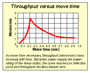
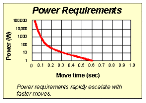
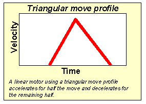
The linear motor Km (Motor Constant, with units of Newtons per root Watt) deserves a closer look. This figure of merit, while the key to linear motor performance, is often missing from vendor data sheets. This constant (for any given motor) relates the ratio between force output (the reason you bought the linear motor) and waste heat generation (an undesirable by-product, which sets the limit on performance). While most advertising claims emphasize the linear motor Kf (the Force Constant, with units of Newtons per Amp), this is largely a free variable, which can be readily changed by altering the coil wire gauge. The Motor Constant Km, on the other hand, is defined only by the copper volume, packing efficiency, and magnetic field strength, and is the true linear motor quality factor. Km is also particularly helpful when it comes to calculating system performance. This value varies with the motor size and design, and typically ranges from 5 to 25 N/W0.5 – larger numbers offer higher performance, are physically larger, and cost more due to the increased magnet and coil volume. In this hypothetical example, the linear motor Km and power rating may have been chosen on the basis of cost, available space, informed motor sizing data, or a “wing and a prayer”. Using the values listed above, let’s run a few numbers on the proposed application. First, we’ll check the top speed against the stated limit, to see if we have any problems on that front. The top speed in a triangular move can be found simply with the formula: Eq.1: V = (2 * X) / t where X is the move size (0.1 meter), and t is the desired move time. This yields a top speed of (2 * 0.1) / 0.10, or 2 meters per second. This is comfortably within the system speed limit of 3.0 meters per second – so far so good. The next quantity to calculate is the acceleration, which is equal to: Eq. 2: A = (4 * X) / t2 where again, X is the move size and t is the move time. This yields an acceleration of (4 * 0.1) / 0.12 , or 40 meters per second squared. Since 9.8 meters per second squared is one “G”, the acceleration in this application could also be referred to as just over 4 “G’s”. Both of the above formulas are not the usual ones that spring to mind when making motion calculations, but are time-saving short-cuts for triangular moves compared to splitting the move into two parts, calculating for half the move, etc. With the acceleration known, the force required falls out from Newtons Second Law: Eq. 3: F = m * A Multiplying the mass (10 kg.) by the acceleration (40 meters/sec2) gives a force of 400 kg-m/sec2 – that is, 400 Newtons. Note that the force is continuous in this application – it applies both during the acceleration phase and (with a direction reversal) during the deceleration phase. The next step, to calculate the power that the linear motor must dissipate, is equally easy: Eq. 4: Power = (Force / Km)2 That is, to calculate the waste heat to be dissipated, simply divide the force by the motor Km (in Newtons per root Watt), and square the result. In this application, the power is (400 / 10)2, or 1600 Watts. Whoops! That’s going to take some kind of honkin’ big (and expensive) motor! Alternately, if the existing 10 N/W0.5 motor (with a continuous power rating of 100 Watts) and 100 millisecond move time were to be retained, the system would require a pause between each move of 1.5 seconds, for a duty cycle of 1:16, or 6.3%. In this example, we intentionally selected values that would require a very high power linear motor. The method works, of course, irrespective of the actual numbers used, but it would be useful to take a moment to examine the way the system scales, and see how we got into this mess. The simple, yet key insight is to note that, as shown in Eq. 2, the acceleration scales as the inverse square of the desired move time. If we continue to Eq. 4, we see that power scales as the square of the force. Since F = m * A, that’s equivalent to saying that power scales as the square of the mass and/or the acceleration. Now, since acceleration scales as the inverse square of the move time, and power scales as the square of acceleration, we can combine these two to reveal that: Power scales with the inverse fourth power of the desired move time! That is a pretty significant observation. In more explicit terms, the relationship between Power, Move Distance, Move Time, Mass, and the Linear Motor Km is as follows: Eq. 5: Power = (16 * m2 * X2) / Km2 * t We tend to view the world as a fairly linear place, but fourth power laws like this one tend to whack you in the butt before you even see what’s coming. For example, attempting to make a move in one half the time (a reasonable request, coming from a program manager or marketing type) will multiply the linear motor power requirements by a factor of 16!! Similarly, relaxing the time by a factor of two will cut the power requirements by a factor of 16!! in the above application, that would be just enough to let the original motor work properly. Since the move time turns out to be a very “sensitive parameter”, a closer look at how it impacts system performance is in order. To assemble this last piece of the puzzle, let’s explore what happens to not just system power, but throughput (expressed in moves per second), as we vary the move time. Obviously, if we make the move time very long, the number of moves per second will be greatly reduced. For example, if we take one full second to make the above move, we can pretty much count on a throughput of one move per second. As we slowly shorten the move time, the number of “moves per second” – we’ll abbreviate this as “MPS” – rises inversely with the move time. If we were to graph this function, it would be the standard k/t curve – a hyperbola. What is not glaringly obvious is that this smooth curve runs into serious trouble as soon as the power equals the power rating of the linear motor. At this point, our smooth curve encounters a “discontinuous inflection point”, and the MPS begins an inverse cubic power crash towards zero! This is clearly shown in the graph of Fig. 2, where the two very different regions of the curve are readily apparent. In our example, the MPS will be a paltry 0.6 at our chosen move time of 100 milliseconds. In Fig. 3, the rapidly escalating power requirements associated with short move times are also graphed.

Figure 2 – Moves/Second vs. Move Time

Figure 3 – Power vs. Move Time
The cause of this discontinuity is fairly simple to understand. As soon as the continuous power rating of the linear motor coil is reached, any further reduction of the move time will require longer and longer “cooling off spells” to allow the excess power to dissipate. Despite the intuitive conclusion that this delay is canceled by the reduction in the move time, the fourth power nature of the relationship stymies our common sense, and leads to vastly lower MPS. The decrease in move time does help a little, reducing the fourth power term to a cubic one, but this is little consolation. The most important observation to draw from this is that for any given system, there exists an optimum move time, which may well be longer than one would expect. If you find yourself on the left-hand side of the cusp, then you will actually increase the MPS, and hence productivity, by allowing the move time to increase. You truly can “Slow Down to Speed Up”! In our above example, slowing down the move time from 100 to 200 milliseconds will increase the MPS from 0.6 to 5.0 – an 800% improvement! The number of variables that determine the optimum move time are actually quite few – namely, the moving mass, the move distance, and the linear motor Newtons per root Watt. We have seen a number of examples of systems in which the move time was selected based on the goal of a certain number of parts per hour, or an overall cycle time was chosen, and then allocated among the machine operations with little or no attention to proper motor sizing. In some cases, the inevitable “cooling off pauses” are inserted automatically by motor coil thermal sensors or an amplifier “I2T” function, and the only obvious signs of a problem are that the system is sluggish and “not meeting spec”. In other cases, technicians pad in delays on an empirical basis until the linear motor coils “stop burning out”. For our simple example, it would be fairly easy to size the motor properly so as to operate at the desired throughput. In real-world systems, however, with considerably more complex motion sequences, it is a rare designer who prepares a detailed power model of the complete system. Additional constraints can include the cost of linear motors, or even the amount of space available to fit the motor. By the way, the concepts expressed in this article also apply to rotary motor systems, although in this case the moment of inertia of the motor rotor and leadscrew often predominate over the reflected payload mass. In conclusion, it’s clear that the inverse fourth power relationship between power and move time requires that we carefully consider cycle times and motor sizing when designing motion systems. The square law between moving mass and power similarly requires effort to minimize the moving mass. Casual comments such as “We need to slice 100 milliseconds off the cycle time” need to be evaluated in light of the potentially expensive underlying physics. Finally, the fact that the productivity curve has such a pronounced maximum can help us to more thoughtfully design systems that operate at peak performance. “Slow Down to Speed Up!” is the first in a series of provocative essays; subsequent titles under consideration include “Spend your Way to Riches!”, and “Up is Down!”.
Motion Control Handbook
Abbé Error
Accuracy in Positioning Systems
Constant Velocity
Cosine Error
Full Coil vs. Half Coil
Glossary of Terms
High Vacuum Positioning Tables
Interferometer Feedback Systems
Interpolated Motion
Lead Screws and Ball Screws
Linear Motors
Limit Sensors
Limitations of Piezos
Low Magnetic Field Tables
Linear Positioning Accuracy
Mapping
Microstepping
Midrange Resonance
Motion Calculations
Mounting Issues
Move and Settle Time
Positioning Systems Overview
Repeatability
Resolution
Rotary Motor Mount
Servo Motors
Slow Down to Speed Up
Stepper Motor
Thermal Expansion
Torque and Force Requirements
Units of Measure
Vibration Isolation Systems

