Automated Digital Microscopes and Optics Optimization
At the heart of many biomedical instruments lies an automated digital microscope. While many of these systems employ simple brightfield imaging with epi (through the objective) illumination, variants include transmissive illumination, fluorescence microscopy, darkfield illumination, TIRF, Nomarski, confocal, etc. In all of these cases, some simple optical rules can be used to optimally configure a system for your application, and these rules in turn drive the requirements for the system’s mechanics. In this article, we’ll explore how the optics and mechanics interact, and show you some ways to optimize your imaging throughput.

What is Optical Instrument Resolution
The first step is to determine how much optical resolution your system needs. A simple mammalian cell counting application might be fine with a resolution of 2 µm, while a pathology application targeting fine structural morphologies of cell nuclei might need 0.35 µm resolution. A key property of any microscope objective is its NA (Numerical Aperture), which is the sine of the half angle of the cone of light passing through the objective. The proper NA for an application is equal to 0.5 λ/R, where λ is the wavelength of the illumination (typically 0.5 µm), and R is the desired resolution, in the same units. That cell counting application requires an NA of only 0.12, while the pathology application would require an NA of 0.70.


How to Calculate Numerical Aperture and Why it’s Important
With the NA chosen, the objective’s magnification is no longer a free variable. The higher the NA, the higher the objective’s magnification will be. Typical NA ranges for microscope objectives are as follows: 4X: 0.1 to 0.2; 10X: 0.25 to 0.4; 20X: 0.4 to 0.8; 40 and 60X: 0.65 to 0.95. In general, higher NA objectives within a given magnification are more expensive, but provide higher resolution. Let’s assume for this article that your required resolution is 0.4 µm, and that you have chosen a 20X, 0.70 NA objective. The next choice that you will need to make is whether the objective has finite conjugates, or is infinity corrected. If no optical elements are needed between the objective and the sensor, a finite conjugate objective can be used (typically with a 160 or 210 mm tube length), but in many cases, a beamsplitter, fluorescent filter cube, or other optical element is needed between the objective and the sensor. In this case, you will need to select an infinity corrected objective, and add a tube lens between the last optical element and the sensor. Tube lenses typically have unity magnification, but other powers are available, and allow you to tweak the overall magnification. The total magnification equals the objective magnification times the tube lens magnification.


With the magnification chosen, we can now address the field of view (FOV) at the biological sample. This is simply the imaging sensor size, divided by the magnification. For example, if the image sensor is 10 mm square, and the magnification is 20X, then the FOV will be 0.5 mm square. Your typical biological sample, whether the canonical 25 x 75 mm glass slide, a tissue section, or a custom flow cell, will be many times larger than this field of view. A programmable XY stage allows many small fields of view across the total area of your sample to be imaged sequentially moving quickly from one FOV to the next. It isn’t practical to simply take a single giant image, as image sensor costs soar as they get larger, and microscope objectives are at most corrected for a 25 mm image diameter (the diagonal of a 17.7 mm square image sensor).

High Throughput Imaging XY Stages
The job of the XY stage is two-fold: to accurately and as quickly as possible jump from one FOV to the next, and to settle very quickly at the new FOV, with any residual vibration well under the optical resolution. As soon as the stage has settled to within the optical resolution, image exposure begins, and as soon as the image integration is complete, the stage jumps to its new FOV, while the digital camera downloads its image to the host. The travel of the XY stage should at least equal the length and width of your sample, and additional travel may be required to permit sample loading and unloading. There are a number of ways to implement an XY stage, with varying levels of performance. For low throughput applications, a stepping motor and a leadscrew will be adequate. Time must be budgeted after the end of each move for the high-Q ringing of the payload mass and nut/bearing compliance to damp out. Direct drive stages with linear servo motors and linear encoders provide the highest levels of performance. For a typical move size (FOV) of 0.75 mm, a direct drive stage such as the Dover Motion MMX series can move and settle to under 0.5 µm in about 50 milliseconds. Depending on the integration time of the digital camera and the illumination intensity, this can permit as many as 16 images per second to be acquired. The actual (not empty) resolution of the XY stage must be several times finer than the optical resolution; in the above 20X, 0.70 NA example, the stage resolution should be at least 0.1µm.
Determining Pixel Size
The image sensor consists of millions of individual pixels, and a good rule of thumb is to choose a pixel size such that the optical resolution corresponds to between 1 and 2 pixels at the image sensor. For our 20X, 0.70 NA example, with a resolution of 0.4 µm, we simply multiply this resolution times the magnification (20X) to get 8 µm; sensor pixels of from 4 µm to 8 µm would be suitable for this application.
Calculating Depth of Field
Our next task is to make sure that the sample is precisely focused, and this requires that we calculate the depth of field (DOF). This is the distance along the optical axis that we can move the sample from precise focus, and still be able to fully resolve fine details in the sample. For a given NA, and with air between the objective and the sample, the DOF will be:
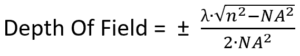
Where NA is the numerical aperture, and λ is the wavelength of light (typically 0.5 µm).
In almost every case, an automated Z axis objective positioner is required to maintain focus across the sample. For low NA objectives, such as a 4X 0.15 NA, the depth of field is a whopping 22 µm, and a simple leadscrew based stage, or even a cam will be suitable for moving the objective into precise focus. For high NA systems, however, the demands are much more stringent; for a 20X, 0.80 NA apochromatic objective, the depth of field is only +/- 0.48 µm. This level of precision requires a higher level of Z stage performance, and again, direct drive stages such as the Dover Motion MMX, with 5 nanometer resolution, are more than up to the task.

Our final task is to know what position to command of the Z focus axis to ensure precise focus. For thin samples, one technique is to use a continuous tracking laser autofocus system, directed down through the objective by a beamsplitter. Such a system can detect the reflection off the underside of a coverslip, and an optical coating on this surface can be designed to pass visible light while strongly reflecting the IR wavelength of the laser autofocus. For thick samples, it may be necessary to acquire images at multiple planes within the sample, and choose the image with the highest contrast. The ultimate technique to increase image throughput, if your budget supports it, is to add additional cameras. The image below shows the objective end of a four camera system, with four 20X, 0.80 NA objectives on 36 mm pitch, each on its own direct drive focus axis (MMX), and each with its own continuous tracking laser autofocus. This system is capable of acquiring and processing 350 million pixels per second!

Acquiring images of biological samples is complex, and is increasingly required in a wide variety of diagnostic tools. Getting the workflow right requires close collaboration across several technical disciplines, but if you follow some simple rules to ensure both the optic and mechanical design elements align with the application requirements, you will be well on your way to project success.
Related Products

The DOF™ microscope stage is optimized for objective focusing with increased travel, higher bandwidth, and lower cost than piezo stages.
| wdt_ID | Travel | 5-9 mm |
|---|---|---|
| 1 | Resolution | 1.25 nm |
| 2 | Repeatability | < 50 nm |
| 3 | Bandwidth | > 225 Hz |

The award winning SmartStage™ XY stage offers high precision and includes an embedded controller inside the stage.
| wdt_ID | Travel | 50 - 200 mm |
|---|---|---|
| 1 | Accuracy | ≤ 10 μm |
| 2 | Repeatability | 0.8 μm |
| 3 | Payload | 10 kg |
