Automated Imaging
What is Automated Imaging?
Many modern high-technology products and processes depend on the control and visualization of things that are very small. Because of this, automated imaging is one of the most common applications for XY stages. In this application, microscopic attributes of a macro object are examined by moving it in two axes relative to a high magnification imaging system. In this article, we’ll discuss:

XY Imaging Configurations
A popular method for small to medium sized samples is to move the sample in both the X and Y axes under a stationary imaging axis. In these XY imaging configurations, the imaging axis is often mounted to a stationary bridge or a stiff, cantilevered support structure. This move-the-sample approach becomes significantly more challenging as the sample size increases. An example of a system in which the sample moves in two axes is a planar XY stage. Unlike simpler systems where the two axes are stacked on top of each other, the planar XY stage uses air bearings to float the sample carriage above a flat surface that is typically made of granite. At the other extreme, the sample can be stationary while the imaging axis moves in 2 axes, as seen in Figure 2.

For small systems, the imaging system can simply be mounted to its own XY table. In larger systems, the imaging axis typically moves along an overhead bridge in one axis while the bridge itself moves in the other axis. While short bridges can be driven on only one side with a guideway that is stiff in yaw, it is more common to drive and encode both sides of the bridge in what is called “gantry” operation.
Split-Axis Imaging
A popular method for small to medium sized samples is to move the sample in both the X and Y axes under a stationary imaging axis. In these XY imaging configurations, the imaging axis is often mounted to a stationary bridge or a stiff, cantilevered support structure. This move-the-sample approach becomes significantly more challenging as the sample size increases. An example of a system in which the sample moves in two axes is a planar XY stage. Unlike simpler systems where the two axes are stacked on top of each other, the planar XY stage uses air bearings to float the sample carriage above a flat surface that is typically made of granite. At the other extreme, the sample can be stationary while the imaging axis moves in 2 axes, as seen in Figure 2.
Key System Parameters

Automated imaging spans across many industries. The macro objects being imaged can include fluorescent amplicons in a DNA sequencer, stained or labeled cells and tissue samples in diagnostic/life science instrumentation, fine pitch features on a semiconductor wafer, and thin-film transistors in an LCD display. A few key attributes allow us to design optimal positioning systems with automated imaging: field of view, magnification and numerical aperture, imaging resolution, and depth of field.
Field of View The field of view (FOV) is the size of the area able to be captured by the automated imaging system at one time. In an optical imaging system, the FOV equals the image sensor dimensions divided by the total magnification. For example, with a CMOS sensor that is 14 by 16 millimeters, and with a total magnification of 20X, the field of view will be 700 by 800 microns. The sample being imaged by the system is generally many times larger than the FOV, and this is where the XY stage comes in. Its mission is to image some or all of the sample by moving it and the imaging system relative to each other in two axes while acquiring numerous images of individual fields of view.
Magnification and Numerical Aperture The magnification in an automated optical imaging system is generally determined by the choice of objective. Though in infinity corrected optical systems, the total magnification will be the product of both the objective and the tube lens magnifications. As described above, the imaging sensor size and the total magnification determine the FOV in optical imaging systems. The objective’s numerical aperture (NA) is equally as important as the magnification because it is key to the resolving power. The NA is equal to the sine of the half-angle of the cone of light entering the objective, and sets the system’s optical resolution.
Imaging Resolution Imaging resolution can vary over a wide range and is key to determining the appropriate level of stage technology to deploy in any given application. In automated optical systems, there are 2 resolutions to consider: the geometric resolution and the optical resolution. Geometric resolution is simply the FOV size divided by the number of pixels in the image sensor. In the previous example (a FOV of 700 x 800 microns), if the imaging sensor had 2800 x 3200 pixels, the geometric resolution would be 0.25 microns. The optical resolution is set by diffraction theory—it is equal to the wavelength of light, divided by a NA of 2. As an example, for yellow light (0.55 micron), and an NA of 0.5, the optical resolution will equal 0.55 micron. If the geometric resolution is coarser than the optical resolution, you are throwing away resolution. At the other extreme, a geometric resolution considerably finer than the optical resolution provides no additional information. The best compromise is typically a two-fold oversampling, with the geometric resolution being 2 times as fine as the optical resolution. We pay careful attention to the optical resolution since it sets the performance requirement for the X and Y positioning axes. Our goal is to select a stage technology which delivers position resolution that is at least 5 times finer than the optical resolution. Applications vary widely with respect to imaging resolution and appropriate stage technology, as shown in Figure 3.

| Imaging Application | Imaging Resolution | Stage Technology |
|---|---|---|
| Low NA microscopy | 1 to 5 microns | Stepping motors and lead screws |
| Medium NA microscopy | 0.5 to 2.0 microns | Lead screws or linear motors |
| High NA microscopy | 150 to 500 nanometers | Linear motors and linear encoders |
| Hyper-resolution, scanning electron, and helium-ion microscopy | 3 to 50 nanometers | Linear motors and linear encoders |
| Atomic force microscopy | 10 – 20 picometers | Linear motors with Coulomb friction |
Figure 3: Typical imaging applications with resolution and stage technology In low magnification systems with low NA optics, simple open loop stepping motors with a microstepping drive can provide more than adequate position resolution and stability. They also provide reasonable throughput in moving from field to field. As the NA and/or imaging throughput increases, direct drive solutions with linear motors and linear encoders are the stage technology of choice. For advanced microscopy applications, sine/cosine output encoders with arc-tan interpolation provide a valuable increase in position resolution. This technique allows a resolution of 1.22 nanometers with 20-micron pitch encoders, and with fine pitch (0.25 micron) encoders the resulting resolution is extremely low at 15 picometers. To put this into perspective, the classical Bohr diameter of the hydrogen atom is 100 picometers. For the most sensitive applications, such as atomic force microscopy, environmental vibration sets a floor on the position jitter and the Coulomb friction must be engaged to hold still enough during AFM imaging.
Depth of Field Every automated imaging system has a depth of field, which is the range of motion towards or away from the imaging system that will not noticeably degrade the image quality. The depth of field is determined by the wavelength of light and the NA, and it sets the required resolution of the focusing axis. Learn more about focusing on our Focusing Applications and Capabilities page.
Automated Imaging Strategies
There are two fundamentally different ways to perform imaging in two axes; in one case, individual fields of view are acquired sequentially; in the other, the imaging is performed continuously, during constant velocity scanning.
Field-sequential Imaging In field-sequential imaging, the sequence of events is move, stop, image, and repeat. The XY stage moves to its next field of view and stops, the sample remains stationary during image acquisition, and then the XY stage moves to the adjacent field of view. The job of the XY stage is to get to the field on time. The key performance metrics are move and settle time, as well as position jitter during the image acquisition. For low-throughput applications, integrated stepping motor/lead screw assemblies provide a cost-effective solution. When the frames-per-second speed needs to be maximized, linear motors with linear encoders provide the highest performance. An example of a stage that accomplishes this is our MMG™ series of direct drive stages (Figure 5) that supports up to twenty images or “frames” per second at a field of view size of 0.80 millimeters. A random series of fields is sufficient to image and characterize the sample for some applications, and 100% coverage is required in others. In the case of the latter, serpentine stepping is typically the field sequence of choice. In serpentine stepping, the lower mass upper axis moves along adjacent fields of view in a row, after which the lower axis steps to the next row, and the upper axis moves in reverse order down the new row. While the image sensor can be read out during the time that the stage takes to move from field to field, an image is only acquired when the stage is stopped making this a throughput-limited sequential imaging technique. The time spent moving and settling cannot contribute to image acquisition.

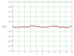 Scanning Imaging Constant velocity scanning imaging is often used when the throughput needs to be maximized and if the image sensor technology can support it. This technique, also referred to as “time delay and integration” (TDI) imaging, generally requires a charge-coupled device (CCD) sensor that will be continuously illuminated while images are continuously acquired. The use of constant velocity imaging results in a huge improvement in imaging throughput. The scan axis moves at a constant velocity in TDI imaging so that the light from any given point on the sample arrives on a succession of photosites in the image sensor and slowly builds in brightness as the photoelectrons are shifted row by row across the face of the CCD sensor. For a detailed review of how CCD sensors work, and how they can be used with constant velocity scanning stages for TDI imaging, read our white paper on biomedical imaging here. In TDI imaging, the speed of stage motion is synchronized with the clocking of vertical transfers in the CCD imager. Our preferred approach is to use a linear encoder on the scan axis to trigger vertical transfers in the imaging sensor. This relaxes but does not eliminate the requirement for extremely constant velocity, since variations in velocity can still influence the brightness of the image. We have made extremely constant velocity motion a priority for decades, leveraging improvements in air bearings, crossed roller guideways, position feedback, and electronic drive and control, to provide exceptional levels of performance. In Figure 6, a constant velocity scanning stage displays position tracking errors of ± 5 nanometers. The low-period errors are measurement artifacts due to atmospheric pressure changes, and the small high-frequency wiggle is cyclical error in the laser
Building the Right Solution for Your Application
Dover Motion offers a variety of standard products for your automated imaging needs, and we also specialize in collaborating with our clients to configure the right motion solution for their unique application. With more than 50 years of experience in the life sciences, diagnostics, and factory automation industries, we understand your automated imaging needs and can provide you the flexibility required to hit your cost and schedule targets. Contact us to learn more about how we can help you with your next project.
Related Products
Learn About Automated Imaging
Automated Imaging Case Studies

The DOF™ microscope stage is optimized for objective focusing with increased travel, higher bandwidth, and lower cost than piezo stages.
| wdt_ID | Travel | 5-9 mm |
|---|---|---|
| 1 | Resolution | 1.25 nm |
| 2 | Repeatability | < 50 nm |
| 3 | Bandwidth | > 225 Hz |

The award winning SmartStage™ XY stage offers high precision and includes an embedded controller inside the stage.
| wdt_ID | Travel | 50 - 200 mm |
|---|---|---|
| 1 | Accuracy | ≤ 10 μm |
| 2 | Repeatability | 0.8 μm |
| 3 | Payload | 10 kg |
